Calculate Statistics of Vegetation Change
To gain insight into the absolute changes in the amount of change, and not just the location of it combined with a visual assessment, it is possible to calculate the percentages of vegetation change. The following example calculates these, and proceeds to plot it, both in a bargraph and in a change matrix.
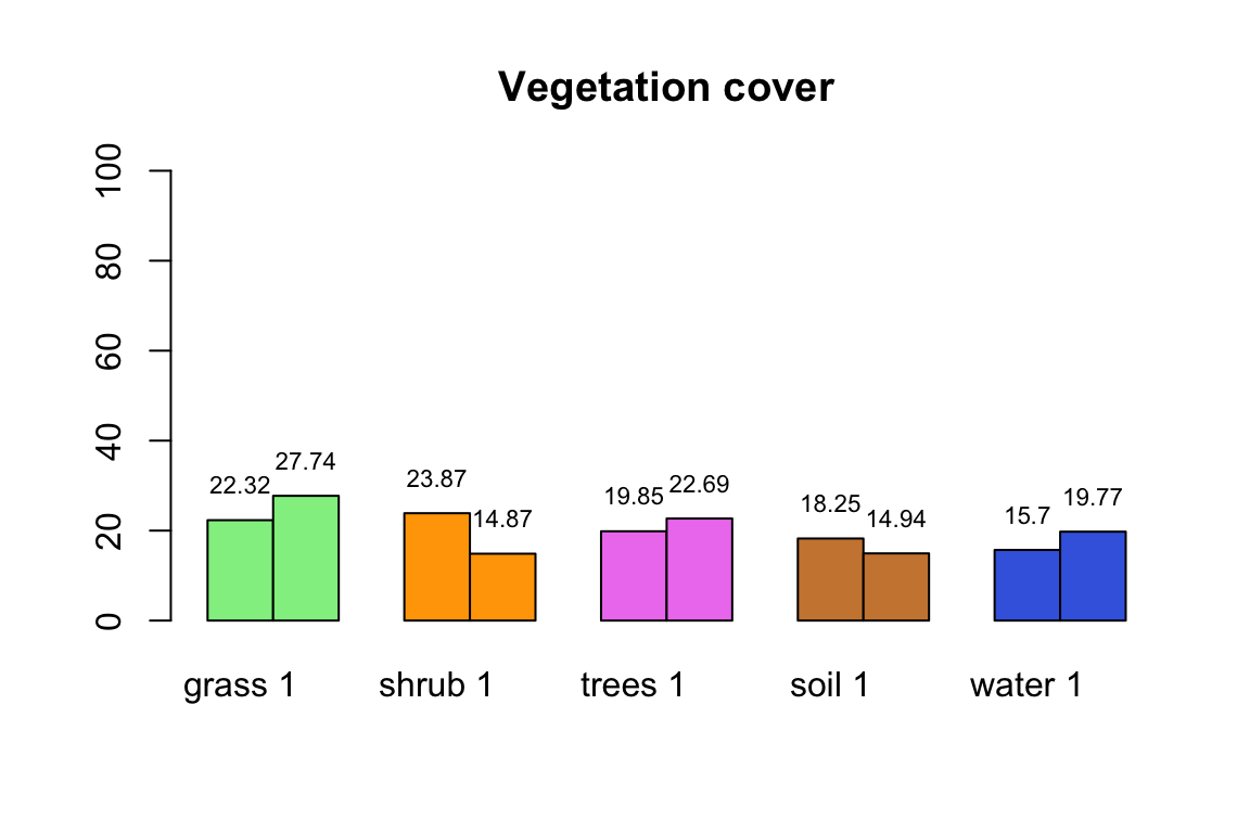
Calculate the Percentage of each Vegetation Cover During each Year
First, we calculate the percentage of pixels in each vegetation cover class for each year. This is done in the script as shown below. The rasters are imported. Then a loop is build in order to count the number of pixels within each class for both years separately. This is done in a loop, because this way we can get a result of 0 in those classes which have no pixels represented in one or both of the years. That is important, because it will allow us to calculate a 0 percentage cover, instead of non-available data.
Next, the script will sum the amount of pixels as calculated. Using this number as a total area, it proceeds to calculate the percentage of each vegetation class in a vectors for each year.
year_1 = raster("Tutorial_files/veg_klompenwaard_year1.tif", convert = TRUE)
year_2 = raster("Tutorial_files/veg_klompenwaard_year2.tif", convert = TRUE)

# Count stable and unstable pixels
freq_veg_year1 = c()
freq_veg_year2 = c()

for (i in seq(1,5,1)){
  freq_year1 = freq(year_1, digits = 2, value = (i), useNA = "no")
  freq_veg_year1 = c(freq_veg_year1,freq_year1)
  freq_year2 = freq(year_2, digits = 2, value = (i), useNA = "no")
  freq_veg_year2 = c(freq_veg_year2,freq_year2)

}

# Calculate percentage of veg (change) and plot
year1_sum = sum(freq_veg_year1)
year1_per = c(freq_veg_year1/year1_sum*100)
year2_sum = sum(freq_veg_year2)
year2_per = c(freq_veg_year2/year2_sum*100)
The result will be a barplot or a matrix, depending on the users preference, as shown below. ## add matrix
Calculate the Percentage of Stable and Unstable Vegetation
The second part of this tutorial will calculate the percentage of the stable and unstable vegetation from the stability raster which is calculated. This is done in the same way as previously explained for the vegetation types. This time it is not before. done within a loop, because that is not necessary as we will always have some stable and some unstable vegetation.
Again, the user will be able to see a barplot or a matrix of the calculated statistics.
# Import stable map
veg_stable = raster("klompenwaard_stable.tif", convert = TRUE)

# Count stable and unstable pixels
freq_stable = freq(veg_stable, digits = 0, useNA = "no")

# Calculate percentage of stable and unstable pixels
n_stable = freq_stable [2,2]
n_unstable = freq_stable [3,2]
n_total = n_stable + n_unstable

per_stable = (n_stable/n_total)*100
per_unstable = (n_unstable/n_total)*100
Create a Change Matrix
The change matrix can be calculated using the function get_change_stat. It is defined below. As arguments, it takes the the two previously created change raster datasets, the number of classes and the names of the classes. Please note that the lower part of the function aims to restructure the resulting matrix. The calculation is carried out in the first part.
# Load the change rasters
change_raster <- raster("Tutorial_files/changes_binary.tif")
differences <- raster("Tutorial_files/changes.tif")

load("Tutorial_files/leaflets.RData")

# Define the function

get_change_stat <- function(change_raster,differences,nclasses,clas_poly1,clas_poly2){
nclasses_pol2<- length(clas_poly2)
# Count stable and unstable pixels
freq_stable = freq(change_raster)
# Calculate percentage of stable and unstable pixels
n_stable = freq_stable [2,2]
n_unstable = freq_stable [3,2]
n_total = n_stable + n_unstable

per_stable = (n_stable/n_total)*100
per_unstable = (n_unstable/n_total)*100

# Plot distribution of stable and unstable
stability = round(c(per_stable, per_unstable), digits=2)
col = c("lightgreen", "red")


frequencies = c()

for (i in seq(10,nclasses*10,10)){
  for (j in (1:nclasses)){
    freq_change = freq(differences, digits = 2, value = (i+j), useNA = "no")
    frequencies = c(frequencies,freq_change)
  }
}

changematrix2 <- matrix(frequencies,ncol = nclasses_pol2)
colnames(changematrix2)<-clas_poly2
rownames(changematrix2)<-clas_poly1

# Restructure matrix
total <- sum(changematrix2)
changematrix<-cbind(changematrix2,rowSums(changematrix2))
changematrix<-cbind(changematrix,rowSums(changematrix2)/total*100)
changematrix<-rbind(changematrix,colSums(changematrix2))
changematrix<-rbind(changematrix,colSums(changematrix2)/total*100)

colnames(changematrix)[(nclasses+1):(nclasses+2)] <- c("area_m2_year1","area_percent_year1")
rownames(changematrix)[(nclasses_pol2+1):(nclasses_pol2+2)] <- c("area_m2_year2","area_percent_year2")
changematrix[(nclasses_pol2+1),(nclasses+1)]<-sum(changematrix[,nclasses_pol2+1][1:nclasses+1])
changematrix[(nclasses_pol2+2),(nclasses+2)]<-100
changematrix[(nclasses_pol2+1),(nclasses+2)]<-NA
changematrix[(nclasses_pol2+2),(nclasses+1)]<-NA
changematrix<<-round(changematrix,2)

return(list(changematrix,stability))

}
After we defined the function, we only have run it. We write the result in a new object called matrix. The command matrix[[1]] is then used to display the results.
matrix <- get_change_stat(change_raster, differences, nclasses, class_names_1, class_names_2)

matrix[[1]]
## grass sand shrub tree
## grass 285458.00000 297.00000 2506.00000 9425.000000
## sand 3184.00000 152008.00000 0.00000 4713.000000
## shrub 7687.00000 1.00000 147752.00000 3981.000000
## tree 134029.00000 2793.00000 30525.00000 75787.000000
## water 6.00000 900.00000 0.00000 422.000000
## area_m2_year2 430364.00000 155999.00000 180783.00000 94328.000000
## area_percent_year2 40.11981 14.54269 16.85313 8.793536
## water area_m2_year1 area_percent_year1
## grass 0.00000 297686 27.75117
## sand 958.00000 160863 14.99613
## shrub 0.00000 159421 14.86170
## tree 130.00000 243264 22.67779
## water 210135.00000 211463 19.71321
## area_m2_year2 211223.00000 1205375 NA
## area_percent_year2 19.69084 NA 100.00000